Introduction

---

MALER is a user-friendly and easy-to-use web application that helps biologists apply ML models to biological and biomedical data. This page provides documentation on how to use MALER.

MALER provides four types of machine learning analysis, each with multiple model building algorithms, evaluation methods, as well as feature selection methods for users to choose from to build their custom machine learning pipeline. Below is a table summary of our features:

	ML algorithms	Evaluation	Feature Selection	Optimal Feature Subset
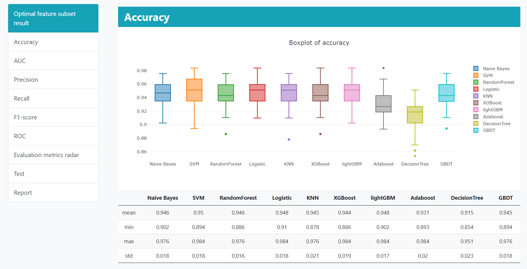
Binary Classification	Naive Bayes, SVM, Random Forest, Logistic Regression, KNN, XGBoost, lightGBM, Adaboost, DecisionTree, GBDT	Accuracy, Recall, Precision, F1-score, AUC	ANOVA(f_classif from sklearn), MRMR(Maximum relevance and minimum redundancy)	Top K, FSS(SFS), BSS
Multiclass Classification
Regression	Linear Regression, SVM, Ridge, Lasso, Decision Tree, XGBoost, AdaBoost, Random Forest, Gradient Boosting Regressor	R-Squared, MAE, MSE	Pearson's correlation (f_regression from sklearn), MRMR(Maximum relevance and minimum redundancy)
Survival Analysis	SurvivalSVM, SurvivalTree, ExtraSurvivialTrees, RandomSurvivalForest, GradientBoostingSurivival	C-index	Univariate Cox regression

Browser and Operating System (OS) Compatibility

---

MALAR is free and open to all users with no login requirement and can be really accessed by a variety of popular web browsers and operating systems as shown below.

Machine Learning Analysis

---

Module selection

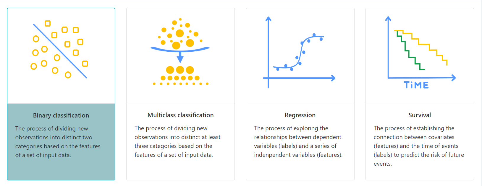
MALER provides four modules including binary classification, multi-class classification, regression and survival analysis. Classification is a supervised process that involves predicting the class of given data points. Regression is a supervised machine learning technique which is used to predict continuous values. Survival analysis aims to predict time to an event.

Data submit

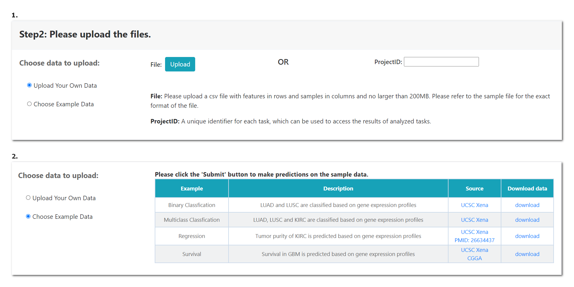
When the module is selected, the user should submit the corresponding data format as following. Example data was also provided in “Example Data”.

Format of input files

In general, a feature-by-sample matrix in a csv format is required to initiate the MALER analysis. A sample label file is also suggested to be uploaded so as to evaluate the matrix more comprehensive.

Preview

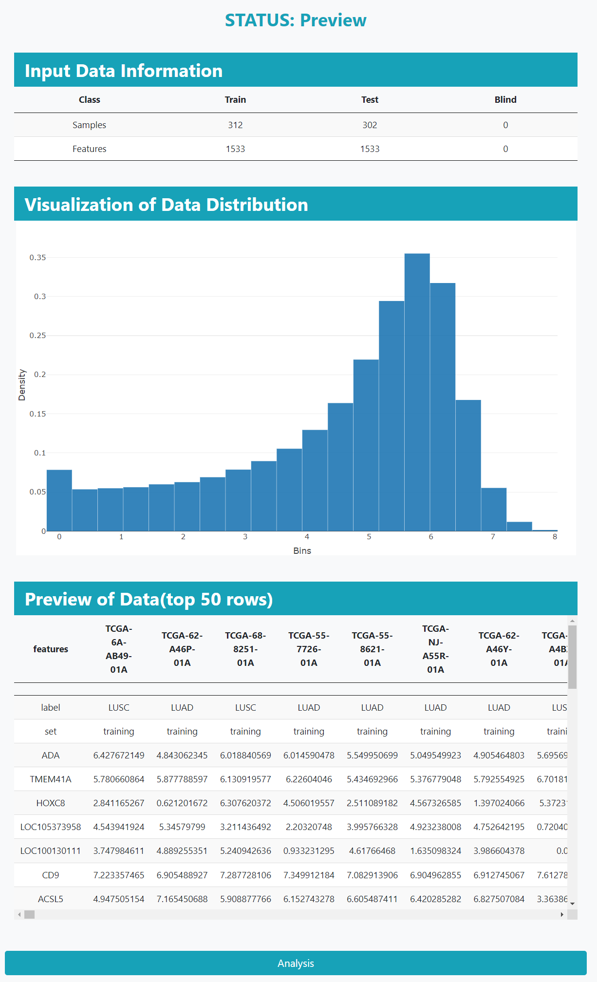
In the preview page, users can view the information and distribution about the uploaded data. After checking the data, click the 'Analysis' button to analyze the input data.

Binary Classification

---

In this module, the sample name, class of samples and ML set are sequentially provided in the first 3 rows of input file. The class of samples indicates 2 sample groups, or “NA” for blind test set. ML set must contain “training”, and can also contain “testing”. Sample data of this data type can be downloaded.

Multiclass Classification

---

In this module, the sample name, class of samples and ML set are sequentially provided in the first 3 rows of input file. The class of samples indicates more than 2 sample groups, or “NA” for blind test set. ML set must contain “training”, and can also contain “testing”. Sample data of this data type can be downloaded.

Regression

---

In this module, the sample name, label of samples and ML set are sequentially provided in the first 3 rows of input file. The label of samples should be continuous/real values as outcome for regression, or “NA” for blind test set. ML set must contain “training”, and can also contain “testing”. Sample data of this data type can be downloaded.

Survival Analysis

---

In this module, the sample name, status, time, and ML set are sequentially provided in the first 4 rows of input file. Time is the follow up time until the event occurs. Status denotes the status of the patient as “dead” or “alive”. The label of samples indicates the information for regression, or “NA” for blind test set. ML set must contain “training”, and can also contain “testing”. Sample data of this data type can be downloaded.

C-index (concordance index): A commonly used metric in Survival Analysis to evaluate performance of prediction models. The C-index is the proportion of concordant pairs (two predictions having same relative order as their true observations) divided by the total number of possible observation pairs. The C-index is widely adopted in survival model performance evaluation, where the order of predicted survival times is compared to the order of the observations.

Time dependent AUC: Calculating the areas under the time-dependent ROC curves results in the time-dependent AUC curve, which is a measure of the discriminative ability of markers at each time point under consideration.

Feature Selection Methods

---

Feature Selection

---

classfication: f_classif ANOVA is performed using the f_classif function from scikit-learn selectKBest package, and features are ranked based on F-statistics.

regression: f_regression Pearson's correlation between each feature and the target is caculated using f_regression from scikit-learn selectKBeset package. The resulting F-statistics and P-values are used for ranking and filtering features.

Multivariate feature selection algorithm: MRMR The MRMR method aims to identify features with the maximum correlation to the target labels while maintaining minimal redundancy among the selected features. Here, we use the F-statistic to assess the correlation between features and the label, while employing Pearson correlation to evaluate redundancy among features.

survival analysis: univariate Cox regression Univariate Cox regression analysis is performed by lifeline package to evaluate the correlation between each feature and survival. And the top 50 features with the lowest P-value were used for follow-up training.

---

Optimal Feature Subset Selection

---

Top K: Top K method selects the first k features from the ordered feature ranking set after univariate feature selection to create the model.

SFS (Sequential Forward Selection): Also called Forward Stepwise Selection (FSS). The method starts with an empty subset of features and appends feature one at a time. During one step, all the features that have not yet been selected are considered for selection, and their evaluation indicator(accuracy) are recorded. At the end of the step, the feature that yielded the best score is included in the subset.Then,a new step is started, and the remaining features are considered. This is repeated this operation until the subset contains 20 variables. Finally, the top k features in the subset with the best performance are selected as the optimal feature subset.

BSS (Backward Stepwise Selection): This method starts with all features included in the model and eliminates one at a time. For each cycle, all the features that have not been eliminated are considered for selection, the feature that yielded the worst score is excluded in the subset. Then, a cycle is started, and the remaining features are considered. This process of deletion and selection is repeated until only one feature is left in the model. Finally, the top k features in the subset with the best performance are selected as the optimal feature subset.

One-click Modeling

---

One-click Modeling allows users run multiple models within the same process. The default parameters would be set for each ML model.

Customized Modeling

---

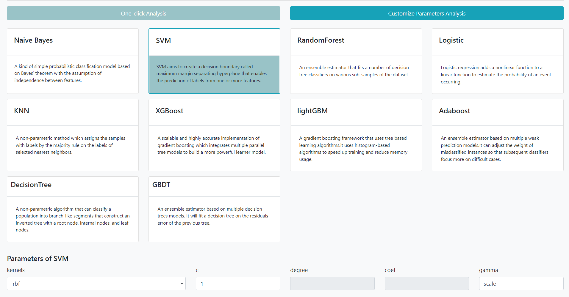
Users can customized the machine learning algorithm using different parameters. The Customized modeling will be stored in the server and could be compared with other modelings derived from the same data under the same ProjectID.

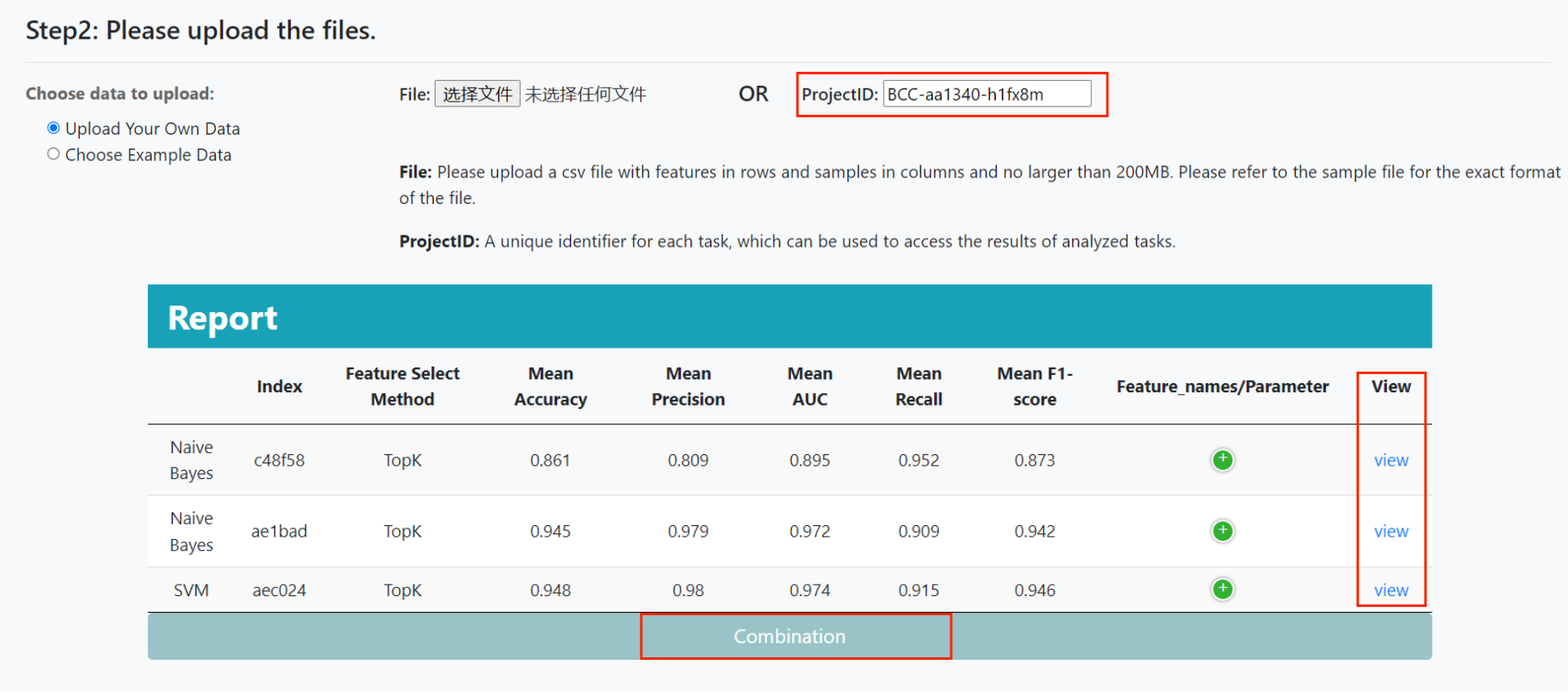
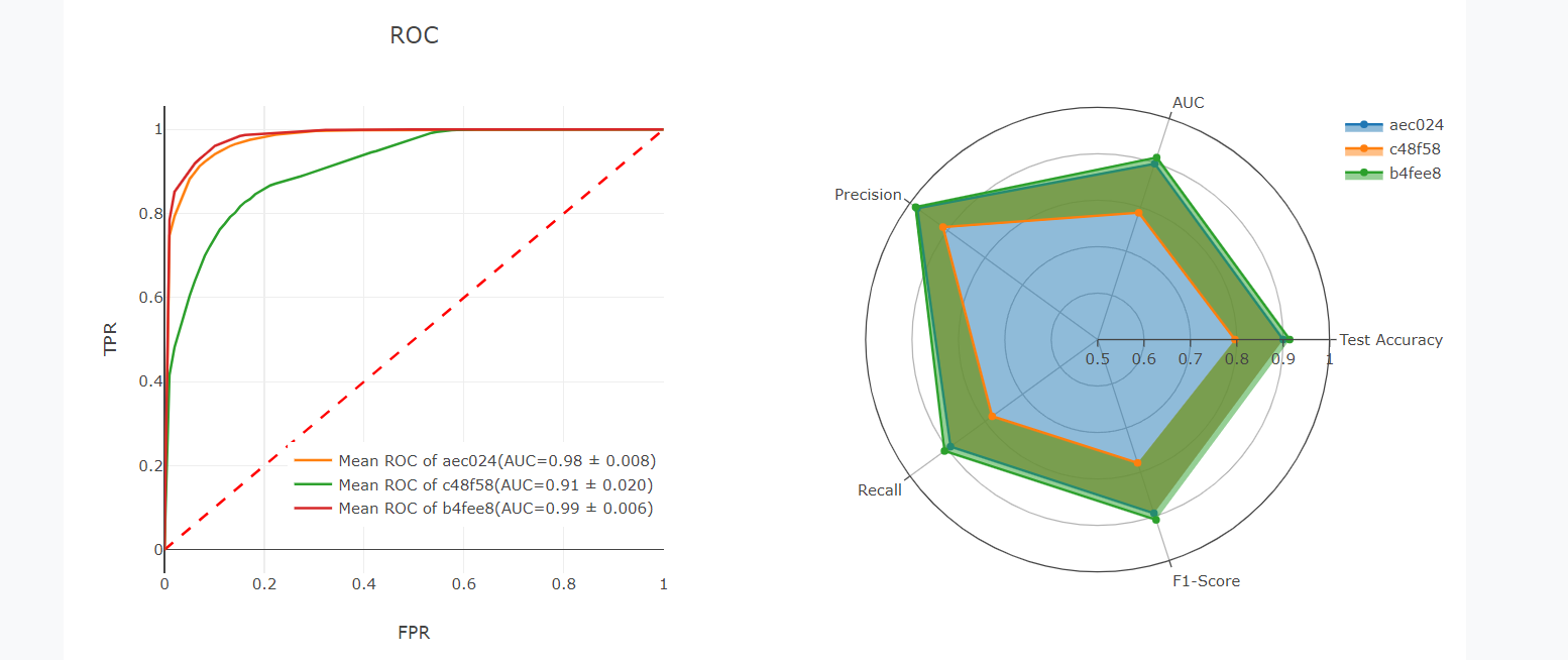
Users can also submit tasks using the same project ID to compare the performance of tasks with different parameters or different models. The results page of the previous task can be returned by clicking the 'view' button, and the 'combine' button can combine the performance metrics of all tasks.

External Prediction

---

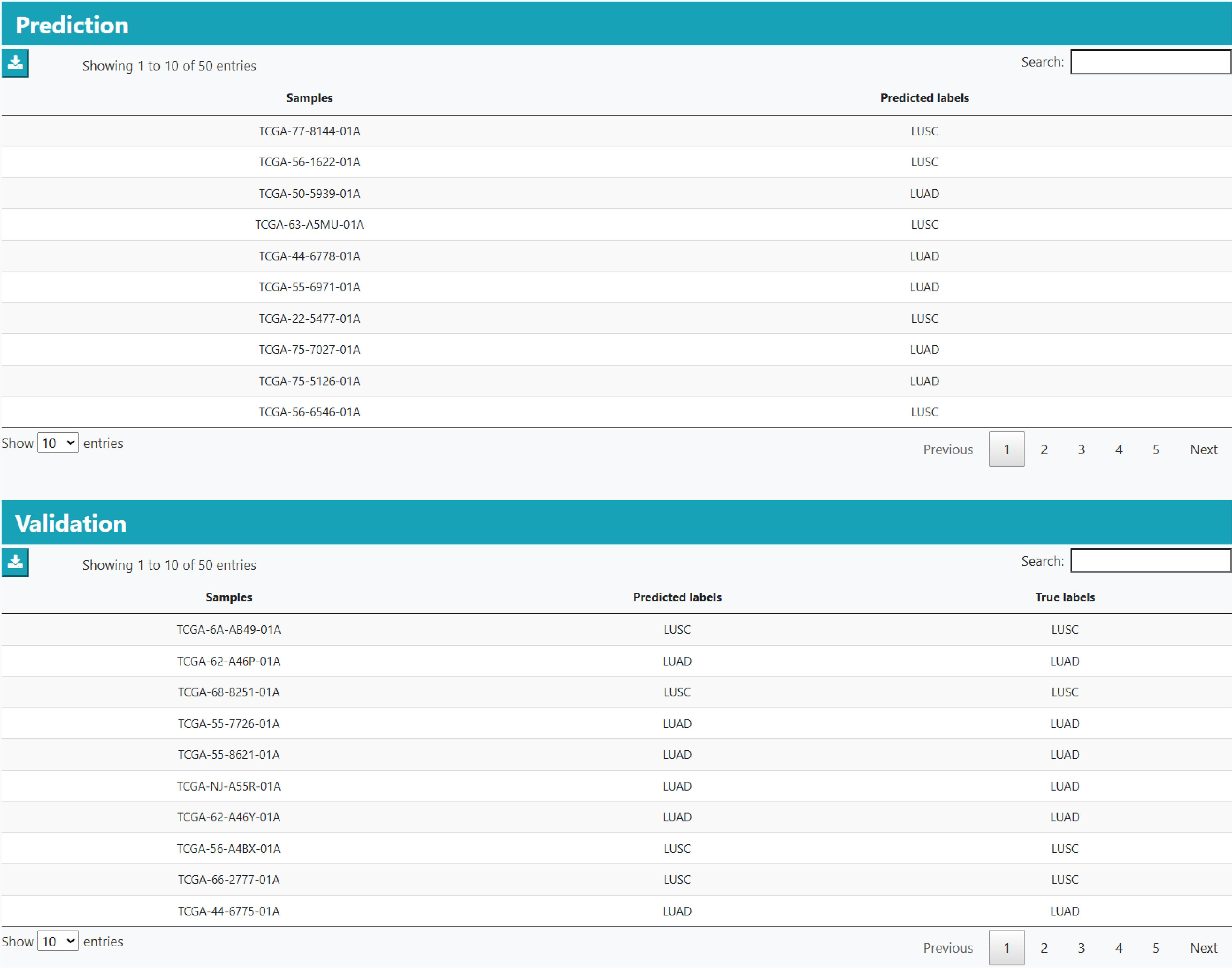
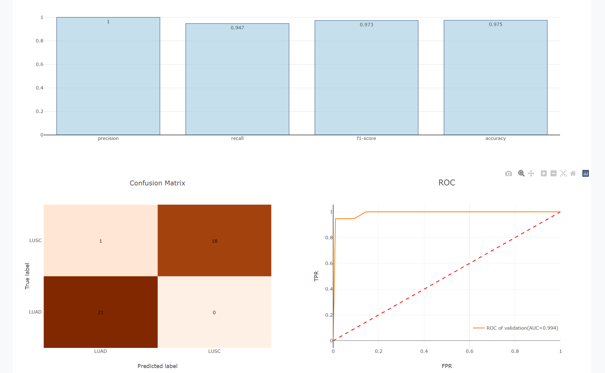
Users can apply the models downloaded from ML Analysis on external data, and performed the prediction. The confusion matrix will be calculated for the validation set, while predictions will be listed in a table for the blind test set.

Sample Data

---

In analysis page, MALER provides sample data to do the analysis using MALER.